
Notes on PCA Theory
These are non-comprehensive notes on the theoretical machinery behind Principal Component Analysis (PCA). This post is essentially an abridged summary of Tim Roughgarden and Gregory Valiant’s lecture notes for Stanford CS1681,2.
Consider a dataset \(\{ \mathbf{x}_i \}_{i=1}^n\) where \(\mathbf{x}_i \in \mathbb{R}^d\) that has been preprocessed such that each \(\mathbf{x}_i\) has been shifted by the sample mean \(\bar{\mathbf{x}} = \frac{1}{n} \sum_{i=1}^n \mathbf{x}_i\). The resulting dataset has a new sample mean equal to the \(\mathbf{0}\) vector.
The goal of PCA is to find a set of \(k\) orthonormal vectors that form a basis for a \(k\)-dimensional subspace that minimizes the squared distances between the data and the data’s projection onto this subspace. This subspace also maximizes the variance of the data’s projection onto it. These orthonormal vectors are called the principal components.
For derivation purposes it is useful to consider finding only the first principal component. Solving for the remaining principal components follows naturally.
For notation simplicity, every time I mention a vector \(\mathbf{v}\) it is assumed to be a unit vector.
Objective Function
The objective function is:
\[\underset{\mathbf{v}}{\mathrm{argmin}} \frac{1}{n} \sum_{i=1}^{n} \big( \text{distance between } \mathbf{x}_i \text{ and line spanned by } \mathbf{v} \big)^2\]Connection to Dot Product
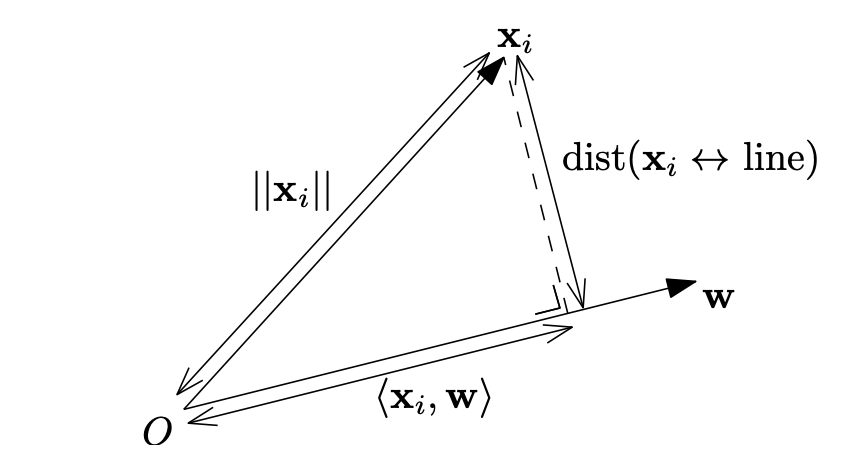
Want to minimize \(\text{dist}(\mathbf{x}_i \leftrightarrow \text{line})\). By the Pythagorean Theorum:
\[\begin{align} ||\mathbf{x}_i||^2 &= \text{dist}(\mathbf{x}_i \leftrightarrow \text{line})^2 + \langle \mathbf{x}_i, \mathbf{v} \rangle^2 \\ \text{dist}(\mathbf{x}_i \leftrightarrow \text{line})^2 &= ||\mathbf{x}_i||^2 - \langle \mathbf{x}_i, \mathbf{v} \rangle^2 \end{align}\]\(\| \mathbf{x}_i \|^2\) is a constant with respect to optimization of \(\mathbf{v}\), so minimizing \(\text{dist}(\mathbf{x}_i \leftrightarrow \text{line})\) is equivalent to maximizing the squared dot product \(\langle \mathbf{x}_i, \mathbf{v} \rangle^2\):
\[\underset{\mathbf{v}}{\mathrm{argmax}} \frac{1}{n} \sum_{i=1}^{n} \langle \mathbf{x}_i, \mathbf{v} \rangle^2\]Note that this maximizes the variance of the projections onto \(\mathbf{v}\).
Matrix Notation and Connection to \(\mathbf{X}^{\top}\mathbf{X}\)
Assemble the \(\mathbf{x}_i\)’s into a matrix:
\[\mathbf{X} = \begin{bmatrix} -\mathbf{x}_1- \\ -\mathbf{x}_2- \\ \vdots \\ -\mathbf{x}_n- \end{bmatrix}\]If we take the inner product of \(\mathbf{Xv}\) with itself, we get the PCA objective function:
\[(\mathbf{Xv})^\top (\mathbf{Xv}) = \mathbf{v}^\top \mathbf{X}^\top \mathbf{Xv} = \sum_{i=1}^{n} \langle \mathbf{x}_i, \mathbf{v} \rangle^2\]The matrix \(\mathbf{A} = \mathbf{X}^\top \mathbf{X}\) is the covariance matrix of \(\mathbf{X}\) and it is symmetric.
The new objective is:
\[\underset{\mathbf{v}}{\mathrm{argmax}} \; \mathbf{v}^\top \mathbf{Av}\]Understanding \(\mathbf{A}\)
Diagonal matrices (ie, zero everywhere except the diagonal) expand space along the standard axes (ie, in the directions of the standard basis vectors).
I won’t prove it here, but an important note for the rest of the derivation is the fact that the solution to \(\mathrm{argmax}_\mathbf{v} \; \mathbf{v}^\top \mathbf{Dv}\) for a diagonal matrix \(\mathbf{D}\) is the standard basis vector corresponding to the dimension with the largest diagonal entry in \(\mathbf{D}\).
Every symmetric matrix can be expressed as a diagonal sandwiched between an orthogonal matrix[source]. The lecture notes consider the case where \(\mathbf{Q}\) is a rotation matrix, but note that orthogonal matrices can take on other forms such as reflections and permutations.
\[\begin{align} \mathbf{A} &= \mathbf{QDQ}^\top \\ \mathbf{X}^\top \mathbf{X} &= \mathbf{QDQ}^\top \end{align}\]This means that symmetric matrices still expand space orthogonally, but in directions rotated from the standard basis.
Eigenvectors
The eigenvectors of a matrix are those vectors that simply get stretched (or scaled) by the linear transformation of the matrix. A vector \(\mathbf{v}\) is an eigenvector of matrix \(\mathbf{A}\) if the following equality holds:
\[\mathbf{Av} = \lambda \mathbf{v}\]Where \(\lambda\) is the eigenvalue associated with \(\mathbf{v}\), which indicates how much \(\mathbf{v}\) is scaled (or stretched) by \(\mathbf{A}\).
Now consider the eigenvectors and eigenvalues of \(\mathbf{A}\). We know that \(\mathbf{A}\) stretches space orthogonally along some set of axes. These axes are the eigenvectors, and the eigenvalues tell you how much space is stretched in that direction.
As discussed previously, the solution is the unit vector pointing in the direction of maximum stretch. This is an eigenvector of \(\mathbf{A}\).
Now consider the PCA objective and remember that if \(\mathbf{v}\) is a unit vector and an eigenvector of \(\mathbf{A}\) then \(\mathbf{Av} = \lambda_{\mathbf{v}} \mathbf{v}\) and \(\mathbf{v}^\top \mathbf{v} = 1\):
\[\begin{align} \mathbf{v} &= \underset{\mathbf{v}}{\mathrm{argmax}} \; \mathbf{v}^\top \mathbf{Av} \\ &= \underset{\mathbf{v}}{\mathrm{argmax}} \; \mathbf{v}^\top \lambda_{\mathbf{v}} \mathbf{v} \\ &= \underset{\mathbf{v}}{\mathrm{argmax}} \; \lambda_{\mathbf{v}} \mathbf{v}^\top \mathbf{v} \\ &= \underset{\mathbf{v}}{\mathrm{argmax}} \; \lambda_{\mathbf{v}} \end{align}\]This says the first principal component is the eigenvector of \(\mathbf{A}\) with the largest eigenvalue. The remaining principal components can be found by taking the remaining eigenvectors sorted by their eigenvalues.
References
[1] Tim Roughgarden, Gregory Valiant, CS168: The Modern Algorithmic Toolbox Lecture #7: Understanding and Using Principal Component Analysis (PCA)
[2] Tim Roughgarden, Gregory Valiant, CS168: The Modern Algorithmic Toolbox Lecture #8: How PCA Works