Logistic Regression Deep Dive

Logistic regression is possibly the most well-known machine learning model for classification tasks. The classic case is binary classification, but it can easily be extended to multiclass or even multilabel classification settings. It’s quite popular in the data science, machine learning, and statistics community for many reasons:

• The mathematics are relatively simple to understand
• It is quite interpretable, both globally and locally; it is not considered a “black box” algorithm.
• Training and inference are very fast
• It has a minimal number of model parameters, which limits its ability to overfit

In many cases, logistic regression can perform quite well on a task. However, more complex architectures will typically perform better if tuned properly. Thus, practioners and researchers alike commonly use logistic regression as a baseline model.

Logistic regression’s architecture is a basic form of a neural network and it is optimized the same way as a neural network. This makes it a valuable case study for those interested in deep learning.

In this post I will be deriving logistic regression’s objective function from Maximum Likelihood Estimation (MLE) principles, deriving the gradient of the objective with respect to the model parameters, and visualizing how a gradient descent update shifts the decision boundary for a misclassified point.

Objective Function

Consider a dataset of \(n\) observations \(\{ (x_i, y_i) \}_{i=1}^n\) where \(x_i \in \mathbb{R}^d\) are the observed features and \(y_i \in \{0, 1\}\) are the corresponding binary labels.

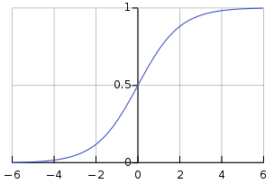
Logistic regression is a discriminative classifier (as opposed to a generative one), meaning that it models the posterior \(p(y \lvert x)\) directly. It models this posterior as a linear function of \(x\) “squashed” into \([0, 1]\) by the sigmoid function (denoted as \(\sigma\)).

The model is parameterized by a vector \(w \in \mathbb{R}^{d+1}\). For notational convenience we will assume each \(x_i\) is concatenated with a \(1\) so that the model’s bias term is contained in the final component of the vector \(w_{d+1}\).

\[p(y=1 \lvert x) = \sigma(w^\top x) \\ \sigma(w^\top x) = \frac{1}{1 + \exp(-w^\top x)} \\\]

Using the notational convenience that \(y \in \{0, 1\}\), we can write the model equation more generally:

\[p(y \lvert x) = \sigma(w^\top x)^y(1-\sigma(w^\top x))^{1-y}\]

Notice the equivalence with the Bernoulli PMF. This means logistic regression is modeling the data with a Bernoulli likelihood. Assuming data are iid, the likelihood of the full dataset is given by:

\[p(y_1, \dots, y_n \lvert x_1, \dots, x_n) = \prod_{i=1}^n \sigma(w^\top x_i)^{y_i}(1-\sigma(w^\top x_i))^{1-y_i} \\\]

There is no closed form solution to logistic regression, so the log likelihood is optimized instead via gradient descent. The log likelihood objective function \(J\) is given by:

\[\begin{align} J &= \log p(y_1, \dots, y_n \lvert x_1, \dots, x_n) \\ &= \log \prod_{i=1}^n \sigma(w^\top x_i)^{y_i}(1-\sigma(w^\top x_i))^{1-y_i} \\ &= \sum_{i=1}^n \log \sigma(w^\top x_i)^{y_i}(1-\sigma(w^\top x_i))^{1-y_i} \\ &= \sum_{i=1}^n \log \sigma(w^\top x_i)^{y_i} + \log (1-\sigma(w^\top x_i))^{1-y_i} \\ &= \sum_{i=1}^n y_i \log \sigma(w^\top x_i) + (1-y_i) \log (1-\sigma(w^\top x_i)) \\ \end{align}\]

Gradient of the Objective Function

In this section, we’ll be deriving the gradient of the objective function with respect to the model parameters \(w\). The derivation makes liberal use of the chain rule and other basic multivariate calculus rules.

The gradient of a sum is equal to the sum of the gradients, so for simplicity let’s consider a single data point.

Simplify notation:

\[\sigma = \sigma(w^\top x)\]

The derivative of the sigmoid function will come in handy:

\[\frac{d}{dz} \sigma (z) = \sigma(z) (1 - \sigma(z))\]

Derivation:

\[\begin{align*} \nabla_w J &= \nabla_w y \log \sigma + \nabla_w (1-y) \log (1-\sigma) \\ &= \frac{y}{\sigma}\nabla_w\sigma + \frac{1-y}{1-\sigma}\nabla_w(1-\sigma) \\ &= \frac{y}{\sigma}\nabla_w\sigma - \frac{1-y}{1-\sigma}\nabla_w\sigma \\ &= \bigg(\frac{y}{\sigma} - \frac{1-y}{1-\sigma}\bigg)\nabla_w\sigma \\ &= \frac{y(1-\sigma) - (1-y)\sigma}{\sigma(1-\sigma)} \nabla_w\sigma \\ &= \frac{y - \sigma y - \sigma + \sigma y}{\sigma(1-\sigma)} \nabla_w\sigma \\ &= \frac{y - \sigma}{\sigma(1-\sigma)}\nabla_w\sigma \\ &= \frac{y - \sigma}{\sigma(1-\sigma)} \sigma(1-\sigma) x \\ &= (y - \sigma) x \end{align*}\]

Visualizing a Gradient Update

A nice property of linear models like logistic regression is that the model parameters \(w\) and the data \(x\) share the same space. Take a look at the gradient:

\[\nabla_w J = (y - \sigma(w^\top x)) x\]

Since \(y\) and \(\sigma(w^\top x)\) are both scalars, the gradient (for a particular data point) is just a scaled version of \(x\). To visualize this, let’s set the stage with a simple 2 dimensional dataset and model. Consider the following binary classification data:

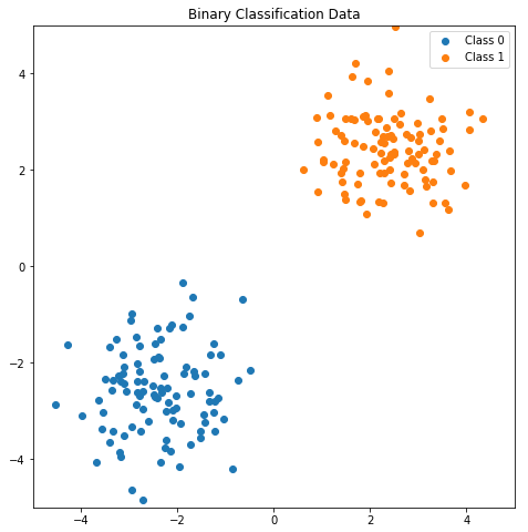
Note: For simplicity in the example below, I’m using a logistic regression model without a bias term. This results in a non-affine decision boundary (ie the hyperplane must pass through the origin).

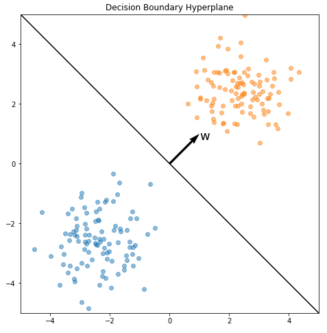
Let’s say the logistic regression model has been trained on this data and has learned model parameters \(w = [1, 1]^\top\). In the default setting (before any threshold tuning), the logistic regression decision boundary is defined by \(p(y=1 \lvert x) = \sigma(w^\top x) = 0.5\), which is equivalent to \(w^\top x = 0\) (you can verify this equivalence by looking at the sigmoid function plot below). This means data is classified as Class 1 if \(w^\top x > 0\) and Class 0 if \(w^\top x < 0\).

In effect, \(w\) defines a hyperplane (the decision boundary) in \(\mathbb{R}^d\), \(H = \{ x \in \mathbb{R}^d \lvert w^\top x = 0 \}\). \(w\) and \(H\) are plotted with the data below.

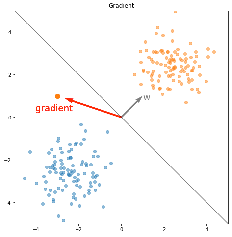
Now, let’s introduce a new data point, \(x = [-3, 1]^\top\) belonging to Class 1 (orange), which is incorrectly classified by the learned model:

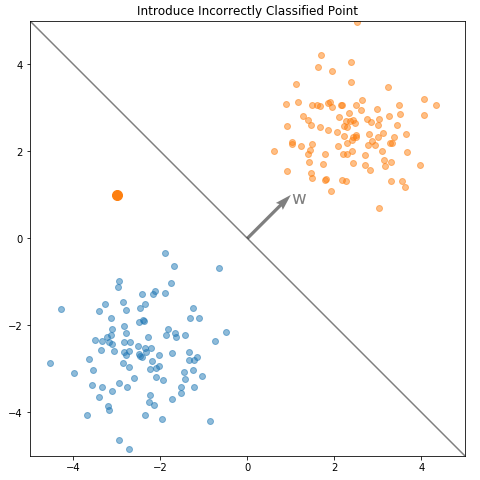
Let’s consider what happens if the model is trained on just this incorrectly classified data point. Computing the gradient:

\[x = \begin{bmatrix} -3 \\ 1 \end{bmatrix} \\ y = 1 \\ \sigma(w^\top x) = \sigma \bigg( \begin{bmatrix} 1 & 1 \end{bmatrix} \cdot \begin{bmatrix} -3 \\ 1 \end{bmatrix} \bigg) = 0.12 \\ y - \sigma(w^\top x) = 0.88 \\ \nabla_w J = (y - \sigma(w^\top x)) x = 0.88 \begin{bmatrix} -3 \\ 1 \end{bmatrix} = \begin{bmatrix} -2.64 \\ 0.88 \end{bmatrix}\]

Now we can plot the gradient alongside the data and the existing decision boundary.

The gradient update equation at iteration \(t\) is

Note: If you’ve seen this equation in the past, the addition sign might throw you off. Usually we minimize the negative log likelihood, but in this case we’re going to maximize the positive log likelihood.

\[w_{t+1} = w_t + \eta \nabla_w J\]

Where \(\eta\) is a learning rate. Let’s compute the updated model parameters:

\[\eta = \text{1e-1} \\ w_{t+1} = \begin{bmatrix} 1 \\ 1 \end{bmatrix} + \text{1e-1} \begin{bmatrix} -2.64 \\ 0.88 \end{bmatrix} = \begin{bmatrix} 0.74 \\ 1.09 \end{bmatrix}\]

Armed with the updated model parameters, we can draw the updated decision boundary:

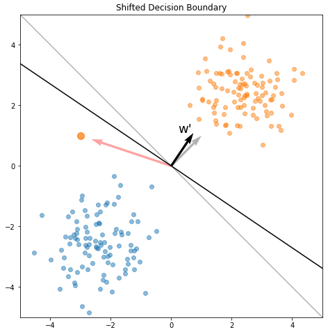
As you can see, adding a fraction of the gradient to \(w\) effectively rotated the decision boundary towards the misclassified point.

Recalling the gradient equation, let’s consider some other cases for the gradient and how we can interpret the math. Hopefully you can visualize how the gradient will attempt to rotate or even “flip” the decision boundary based on the class and location of the data point.

\[\nabla_w J = (y - \sigma(w^\top x)) x\]

description	\(y\)	\(\sigma(w^\top x)\)	\(\nabla_w J\)	comments
model incorrect on a class 1 point	1	0.1	\(0.9x\)	The case illustrated above
model correct on a class 1 point	1	0.99	\(0.01x\)	Model is confident and correct; very small gradient update
model incorrect on a class 0 point	0	0.7	\(-0.7x\)	Rotates (or pushes) the decision boundary the opposite direction
model correct on a class 0 point	0	0.01	\(-0.01x\)	Model is confident and correct; very small gradient update