Getting Up to Speed with SHAP for Model Interpretability

9 minute read

In this post I’ll give a brief overview of SHAP and explain why you should probably add it to your data science toolkit. I’ll also provide some explanation of the basic concepts from game theory that SHAP is built on. The intent of this post isn’t to provide a full treatment of SHAP, but rather to get a practitioner up to speed on the value proposition and theoretical intuition.

SHAP is an effective approach to model interpretability and explainability. It builds on the concept of Shapley Values, which was derived by Lloyd Shapley in the 1950’s. But recent advances in 2017¹ and 2018² papers and the introduction of the SHAP Python library⁶ have brought Shapley Values into mainstream machine learning.

The important issues in model interpretability can be broken down into two parts:

Global Interpretability: Which features are important to my model? Understanding this gives us a better insight into the underlying process that’s being modeled. It’s also useful for feature selection: if a feature is unimportant, remove it. A less well-known but extremely handy use is to check for data leakage.
Local Interpretability: Why did my model make the prediction that it did on a particular data instance (data point)? In many applications, the prediction alone is not enough; it needs to be accompanied by an explanation. In some cases the explanation is required by law. Sometimes the business isn’t interested in the predictions but rather the driving factors; in these cases the model is trained solely for the explanation.

SHAP provides an elegant solution for both. Some data scientists may have experience with using Random Forest feature importances for global interpretability, and instance-level logistic regression activations for local interpretability. SHAP seems to trump these classical approaches in most cases.

From a theoretical standpoint, SHAP is well-grounded and one of the most robust model explanation method out there. SHAP provides some theoretical guarantees that support its trustworthiness: local accuracy, missingness, and consistency. I’ll refer the reader to the excellent references below for more details.

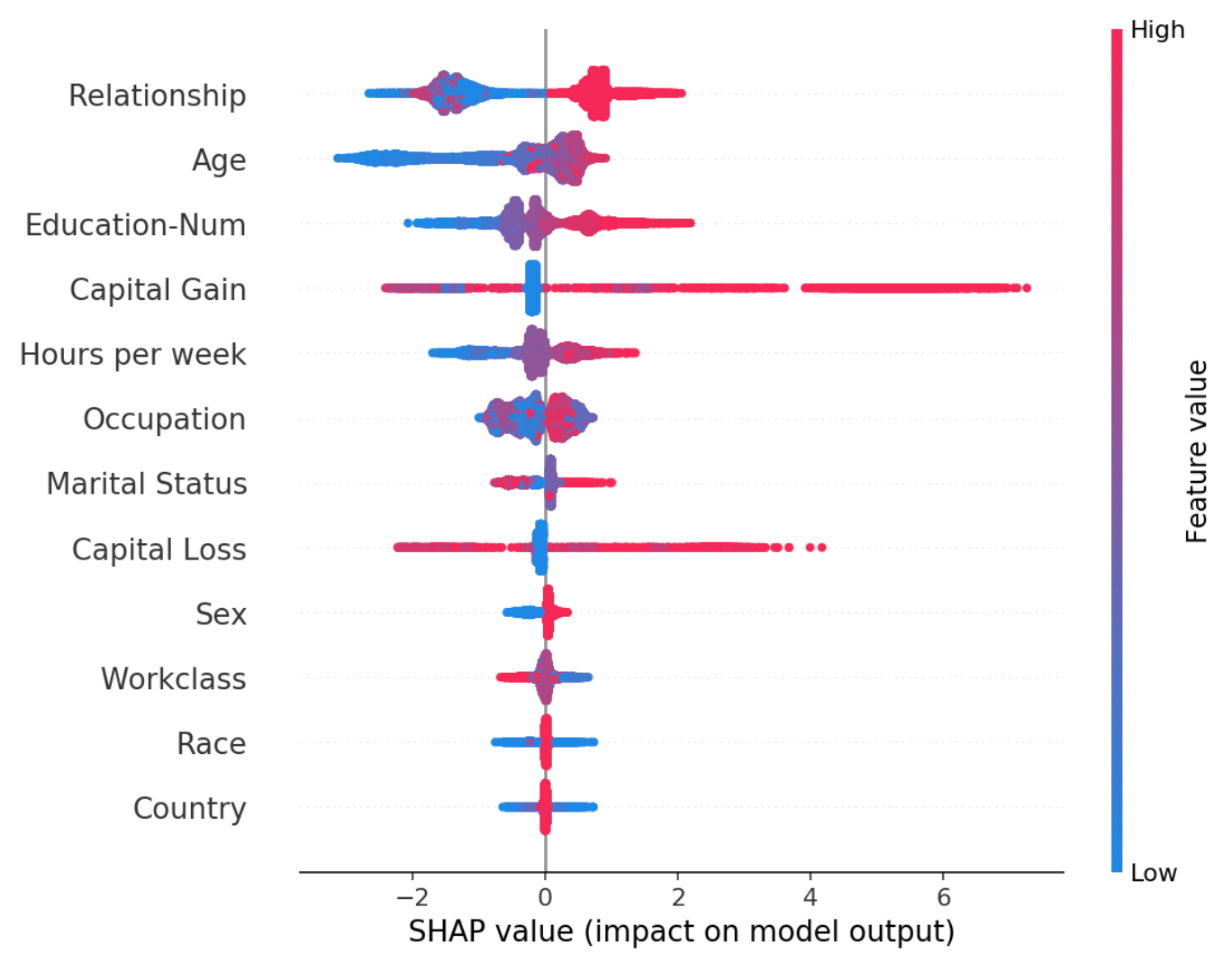
From a practical standpoint, the TreeSHAP implementation is fast and integrates seamlessly with cutting-edge tree-based models like xgboost and lightgbm. The nice integration with highly performant GBT models is perhaps its strongest selling point. You can generate a variety of highly informative plots such as the one shown below. A data scientist can learn much more from these plots than standard feature importance plots (plus, SHAP can generate feature importance plots too).

Sample SHAP Summary Plot⁵

Shapley Values

Here’s the thought experiment that motivates Shapley Values: suppose three people enter a room and play a cooperative game that yields a payout, let’s say $100. Let’s call the players Player A, Player B, and Player C. Assuming each person has a different skillset and contributes in different ways, how should the payout be divided between the players in a fair way? For the purposes of this post, let’s focus on how much payout Player A should receive.

We could approach the problem in an iterative way:

Have A enter the room alone, play the game, and record the payout.
Have B enter the room with A, play the game, and record the payout.
Have C enter the room with A and B, play the game, and record the payout.

The additional amount each player contributed to the payout when they entered the room could be used to split up the winnings. But there’s a problem. Imagine that Player A and Player B have very similar skillsets. Whichever player enters the room first would make a greater contribution because the second player wouldn’t have much more to add. So, maybe we should also look at what happens when B enters first followed by A.

You can see where this is leading. We need to observe all possible combinations of this coalition and average each player’s contribution across them.

Now let’s analyze this a bit further. The figure below shows all possible combinations of the room entry sequence, sorted by when A enters. The coalitions are organized into blocks (via horizontal lines) based on the set of players in the room before and after A enters. It’s important to recognize that the entry order of players who enter before and after A doesn’t matter to A’s calculation. Only the sets matter. For example, there are two coalitions where the set of players $\{B, C\}$ enter the room after A and two coalitions where $\{B, C\}$ enter before A. When computing A’s contribution, it doesn’t matter what order the players enter after A has entered; at this point A has already made its contribution and it isn’t influenced by what what happens next. Similarly, it doesn’t matter what order the players enter the room before A; from A’s perspective, when he enters the room he is playing with the same team whether B came in first or A.

The equation to compute Player A’s Shapley Value is presented below. The set notation and factorials can make this equation daunting at first, so I’ve added some annotation and color coding to assist in unpacking this thing.

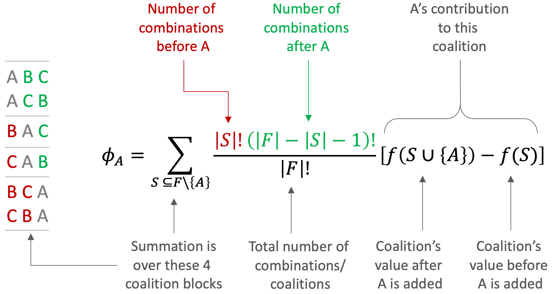
$F$ is the set of all players, so in our example $F = \{A, B, C \}$. The notation $F\setminus\{A\}$ means the set $F$ without $A$ which is $\{ B, C \}$. The value function is represented by $f(\cdot)$, which in our example outputs the payout from a given coalition.

The summation is over subsets $S \subseteq F \setminus \{A\}$. In our example there are 4 subsets/terms in the sum:

\[\emptyset \\ \{B\} \\ \{C\} \\ \{B,C\}\]

As indicated in the annotation, the numerator $\lvert S \lvert ! (\lvert F \lvert - \lvert S \lvert - 1)!$ is the number of combinations of players before A multiplied by the number of combinations of players after A. Ultimately this term computes the number of redundant coalitions where players $S$ enter the room before A, which is the size of the coalition blocks in the figure.

The denominator $\lvert F \lvert !$ computes the total number of coalitions and is used to compute the average contribution of A. One can move $\frac{1}{\lvert F \lvert ! }$ outside of the summation to make this more clear.

After careful unpacking, hopefully it’s more clear now that this equation is iterating over redundant blocks of entry patterns, computing A’s contribution multiplied by the size of the block, and then taking the average.

Application to Machine Learning

The extension of this intuition to machine learning is simple. The players are features in a model, the model is the value function $f(\cdot)$ and the payout is the model prediction. To be clear, the players are instance feature values and the payout is the model’s prediction for that particular instance. For example the players could be the covariates $x = [ age = 45, sex = male, weight = 185 ]$, and the payout could be $f(x) = 0.98$.

While the intuition may be simple, the implementation is quite complex and would be the subject of another post. First of all, if you train a model on a dataset with $p$ features, you can’t directly make predictions with $< p$ features. There are some computationally expensive solutions that require training separate models for each feature subset, but of course that isn’t practical.

This line of thought leads to marginalizing out the effect of feature value subsets and computing expected values over your data, such as³:

\[f(S)=\int f(x_{1},\ldots,x_{p})d\mathbb{P}_{x\notin{}S}\]

And³

\[f(S)=f(\{x_{1},x_{3}\})=\int_{\mathbb{R}}\int_{\mathbb{R}}\hat{f}(x_{1},X_{2},x_{3},X_{4})d\mathbb{P}_{X_2X_4}\]

For the case where there are four features and you’re trying to compute the value of a coalition of only two feature values $S = \{x_1, x_3 \}$.

In practice, a data scientist will likely implement the computationally efficient TreeSHAP² algorithm from the SHAP Python library⁶. This algorithm cleverly exploits the structure of tree-based models such as Gradient Boosted Trees and Random Forests to compute Shapley values efficiently and accurately.

Conclusion

This post introduced SHAP and provided motivation for why a practicing data scientist may want to use it. The primary focus was on building the intuition behind Shapley Values by discussing a simple example and carefully unpacking the Shapley value equation. Finally, the connection was made to machine learning and implementation was discussed briefly.