A Quick Primer on KL Divergence

This is the first post in my series: From KL Divergence to Variational Autoencoder in PyTorch. The next post in the series is Latent Variable Models, Expectation Maximization, and Variational Inference.

---

The Kullback-Leibler divergence, better known as KL divergence, is a way to measure the “distance” between two probability distributions over the same variable. In this post we will consider distributions \(q\) and \(p\) over the random variable \(z\).

It’s beneficial to be able to recognize the different forms of the KL divergence equation when studying derivations or writing your own equations.

For discrete random variables it takes the forms:

\[KL[ q \lVert p ] = \sum\limits_{z} q(z) \log\frac{q(z)}{p(z)} = -\sum\limits_{z} q(z)\log\frac{p(z)}{q(z)}\]

For continuous random variables it takes the forms:

\[KL[ q \lVert p ] = \int q(z) \log \frac{q(z)}{p(z)}dz = - \int q(z) \log \frac{p(z)}{q(z)}dz\]

And in general it can be written as an expected value:

\[KL[ q \lVert p ] = \mathbb{E_{q(z)}} \log \frac{q(z)}{p(z)} = - \mathbb{E_{q(z)}} \log \frac{p(z)}{q(z)}\]

To build some intuition, let’s focus on the following form:

\[KL[ q \lVert p ] = \mathbb{E_{q(z)}} \log \frac{q(z)}{p(z)}\]

Notice that the term \(\log q(z)/p(z)\) is the difference between two log probabilities: \(\log q(z) - \log p(z)\). So, the intuition stems from the fact that KL divergence is the expected difference in log probabilities over \(z\). Although not entirely technically correct, imagine the following to help build an intuition: consider two, perhaps similar, univariate probability density functions \(q(z)\) and \(p(z)\) and imagine sliding across the domain of \(z\) and observing the difference \(q(z)-p(z)\) at every point. This is kind of how KL divergence quantifies the “distance” between two distributions.

Now, a couple of important properties that I won’t prove:

\[KL[q||p] \neq KL[p||q]\] \[KL[q||p] \geq 0 \quad \forall q, p\]

The asymmetric property begs the question: should I use \(KL[q\|p]\) or \(KL[p\|q]\)? This leads to the subject of forward versus reverse KL divergence.

Forward vs. Reverse KL Divergence

In practice, KL divergence is typically used to learn an approximate probability distribution \(q\) to estimate a theoretic but intractable distribution \(p\). Typically \(q\) will be of simpler form than \(p\), since \(p\)’s complexity is what drives us to approximate it in the first place. As a simple example, \(p\) could be a bimodal distribution and \(q\) a unimodal one. When thinking about forward versus backward KL, think of \(p\) as fixed and \(q\) as something fluid that we are free to mold to \(p\).

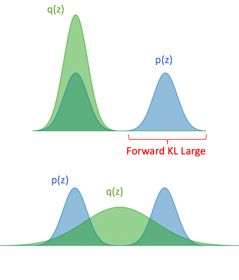
Forward KL takes the form

\[KL[ p || q ] = \sum\limits_{z}p(z) \log\frac{p(z)}{q(z)}\]

As you can see from this equation and the figure below, there is a penalty anywhere \(p(z) > 0\) that \(q\) is not covering. In fact, if \(q(z)=0\) in a region where \(p(z)>0\), the KL divergence blows up because \(\lim_{q(z) \to 0} \log \frac{p(z)}{q(z)} \to \infty\). This results in learning a \(q\) that spreads out to cover all regions where \(p\) has any density. This is known as “zero avoiding”.

Illustration of the "zero-avoiding" behavior of forward KL. Shows a reasonable distribution q with a high forward KL divergence (top), and a different distribution q with a lower forward KL divergence (bottom).

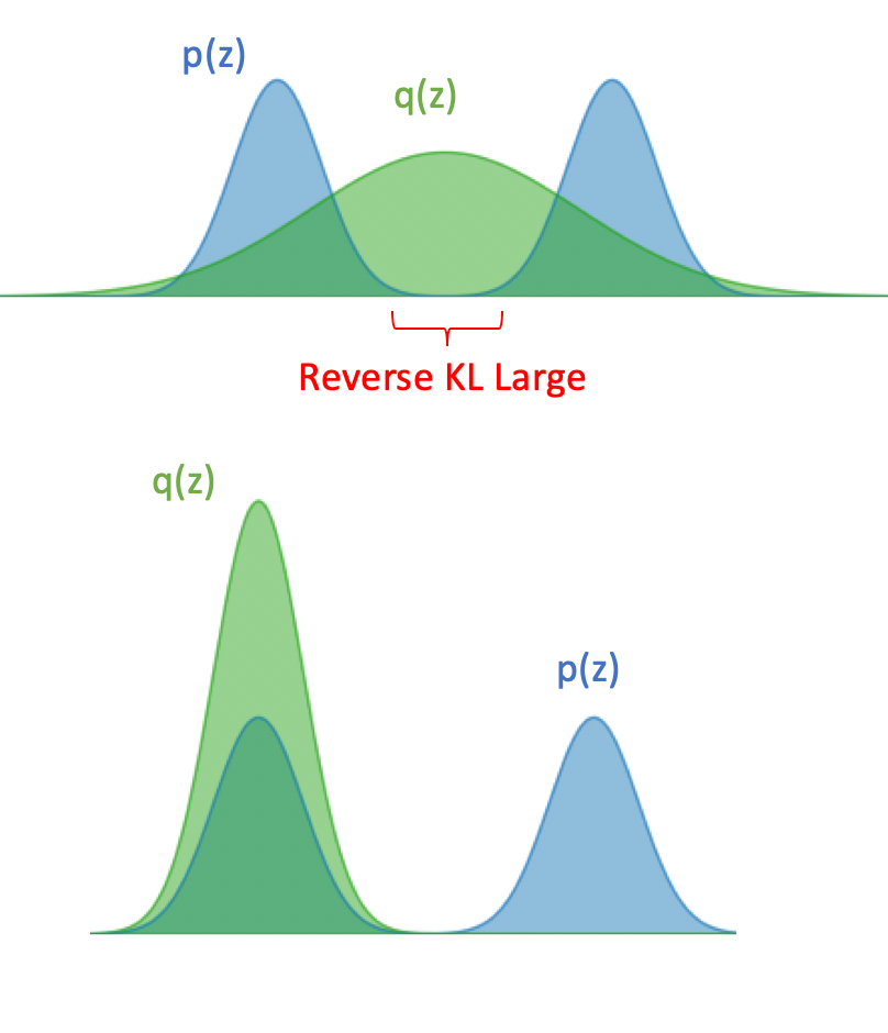
Reverse KL takes the form

\[KL[ q || p ] = \sum\limits_{z}q(z) \log\frac{q(z)}{p(z)}\]

As seen from the equation and the figure below, reverse KL has a much different behavior. Now, the KL divergence will blow up anywhere \(p(z)=0\) unless the weighting term \(q(z)=0\). In other words, \(q(z)\) is encouraged to be zero everywhere that \(p(z)\) is zero. This is called “zero-forcing” behavior.

For example, if \(p\) has probability density in two disjoint regions in space, a \(q\) with limited complexity may not be able to span the zero-probability space between these regions. In this case, the learned \(q\) would only have density in one of the two dense regions of \(p\).

Illustration of the "zero-forcing" behavior of reverse KL. Shows a reasonable distribution q with a high reverse KL divergence (top), and a different distribution q with a lower reverse KL divergence (bottom).

Conclusion

KL divergence is roughly a measure of distance between two probability distributions. There are different forms of the KL divergence equation. You can bring a negative out front by flipping the fraction inside the logarithm. You can also write it as an expectation.

Numerous machine learning models and algorithms use KL divergence as part of their loss function. By exploiting the structure of the specific model at hand, the KL divergence equation can often be simplified and optimized via gradient descent.

KL divergence is asymmetric and it’s important to understand the differences between forward and reverse KL.

My next post builds on KL divergence to explore latent variable models, expectation maximization, variational inference, and the ELBO.

Resources

[1] Eric Jang, A Beginner’s Guide to Variational Methods: Mean-Field Approximation