
Latent Variable Models, Expectation Maximization, and Variational Inference
This is the second post in my series: From KL Divergence to Variational Autoencoder in PyTorch. The previous post in the series is A Quick Primer on KL Divergence and the next post is Variational Autoencoder Theory.
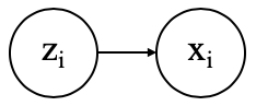
Latent variable models are a powerful form of [typically unsupervised] machine learning used for a variety of tasks such as clustering, dimensionality reduction, data generation, and topic modeling. The basic premise is that there is some latent and unobserved variable \(z_{i}\) that causes the observed data point \(x_{i}\). Here is the graphical model (or Bayesian network) representation:
Latent variable models model the probability distribution:
\[p_{\theta}(x, z) = p_{\theta}(x \lvert z)p_{\theta}(z)\]and are trained by maximizing the marginal likelihood:
\[p_{\theta}(x) = \int p_{\theta}(x \lvert z)p_{\theta}(z)dz\]The introduction of latent variables allow us to more accurately model the data and discover valuable insights from the latent variables themselves. In the topic modeling case we know beforehand that each document in a corpus tends to have a focus on a particular topic or subset of topics. For example, articles in a newspaper typically address topics such as politics, business, or sports. Real world corpora encountered in industry, such as customer support transcripts, product reviews, or legal contracts, can be more complex and ambiguous but the concept still applies. By structuring a model to incorporate this knowledge we are able to more accurately calculate the probability of a document, and perhaps more importantly, discover the topics being discussed in a corpus and provide topic assignment to individual documents.
The learned probability distributions such as \(p_{\theta}(x)\), \(p_{\theta}(z \lvert x)\), and \(p_{\theta}(x \lvert z)\) can be used directly for tasks like anomaly detection or data generation. More commonly though, the main contribution is inference of the latent variables themselves from these distributions. In the Gaussian mixture model (GMM) the latent variables are the cluster assignments. In latent Dirichlet allocation (LDA) the latent variables are the topic assignments. In the variational autoencoder (VAE) the latent variables are the compressed representations of that data.
Marginal likelihood training
Latent variable models are trained by maximizing the marginal likelihood of the observed data under the model parameters \(\theta\). Since the logarithm is a monotonically increasing function, the marginal log likelihood is maximized instead since the logarithm simplifies the computation.
\[\theta = \underset{\theta}{\mathrm{argmax}}\ p_{\theta}(x) = \underset{\theta}{\mathrm{argmax}}\ \log p_{\theta}(x)\]Given a training dataset \(X\) consisting of \(N\) data points \(\{x_1, x_2, \dots, x_N\}\), the marginal log likelihood is expressed as
\[\begin{align} \log p_{\theta}(X) &= \log \prod_{i=1}^{N} p_{\theta}(x_i) \tag{1} \\ &= \sum_{i=1}^{N} \log p_{\theta}(x_{i}) \\ &= \sum_{i=1}^{N} \log \int p_{\theta}(x_i, z_i)dz \\ &= \sum_{i=1}^{N} \log \int p_{\theta}(x_i \lvert z_i)p_{\theta}(z_i)dz \end{align}\]Ideally we would maximize this expression directly, but the integral is typically intractable. For example, if \(z\) is high dimensional, the integral takes the form \(\int\int\int\dots\int\).
As previously discussed, we must also be able to compute the posterior of the latent variables in order to gain utility from these models:
\[p_{\theta}(z \lvert x) = \frac{p_{\theta}(x \lvert z)p_{\theta}(z)}{p_{\theta}(x)}\]Again, this calculation is typically intractable because \(p_{\theta}(x)\) appears in the denominator. There are two main approaches to handling this issue: Monte Carlo sampling and variational inference. We will be focusing on variational inference in this post.
Derivation of Variational Lower Bound
To start, let’s assume that the posterior \(p_{\theta}(z \lvert x)\) is intractable. To deal with this we will introduce a new distribution \(q_{\phi}(z)\). We would like \(q_{\phi}(z)\) to closely approximate \(p_{\theta}(z \lvert x)\) and we are free to choose any form we like for \(q\). For example, we could choose \(q\) to be static or conditional on \(x\) in some way (as you might guess, \(q\) is typically conditioned on \(x\)). A good approximation can be seen as one that minimizes the KL divergence between the distributions (for a primer on KL divergence, see this post):
Note: For simplicity I will be using summations instead of integrals in the derivation.
\[KL[q_{\phi}(z) \lVert p_{\theta}(z \lvert x)] = -\underset{z}{\sum} q_{\phi}(z) \log \frac{p_{\theta}(z \lvert x)}{q_{\phi}(z)}\]Now, substituting using Bayes’ rule and arranging variables in a convenient way:
\[\begin{align} &= -\underset{z}{\sum} q_{\phi}(z) \log \bigg( \frac{p_{\theta}(x,z)}{q_{\phi}(z)} \cdot \frac{1}{p_{\theta}(x)} \bigg) \\ &= -\underset{z}{\sum} q_{\phi}(z) \bigg( \log\frac{p_{\theta}(x,z)}{q_{\phi}(z)} - \log p_{\theta}(x) \bigg) \\ &= -\underset{z}{\sum} q_{\phi}(z) \log \frac{p_{\theta}(x,z)}{q_{\phi}(z)} + \underset{z}{\sum} q_{\phi}(z) \log p_{\theta}(x) \end{align}\]Note that in the second term, \(\underset{z}{\sum} q_{\phi}(z) \log p_{\theta}(x)\), \(\log p_{\theta}(x)\) is constant w.r.t. the summation so it can be moved outside, leaving \(\log p_{\theta}(x) \underset{z}{\sum} q_{\phi}(z)\). By definition of a probability distribution, \(\underset{z}{\sum} q_{\phi}(z) = 1\), so the term ultimately simplifies to \(\log p_{\theta}(x)\). So, we are left with:
\[KL[q_{\phi}(z) \lVert p_{\theta}(z \lvert x)] = -\underset{z}{\sum} q_{\phi}(z) \log \frac{p_{\theta}(x,z)}{q_{\phi}(z)} + \log p_{\theta}(x)\]Rearranging for clarity:
\[\log p_{\theta}(x) = KL[q_{\phi}(z) \lVert p_{\theta}(z \lvert x)] + \underset{z}{\sum} q_{\phi}(z) \log \frac{p_{\theta}(x,z)}{q_{\phi}(z)} \tag{2}\]Now, let’s circle back to Eq. 1. Notice that we have derived an expression for the marginal log likelihood \(\log p_{\theta}(x)\) composed of two terms. The first term is the KL divergence between our variational distribution \(q_{\phi}(z)\) and the intractable posterior \(p_{\theta}(z \lvert x)\). The second term is is called the variational lower bound or evidence lower bound (the acronym ELBO is frequently used in the literature).
\[\begin{align} \mathcal{L} &= \underset{z}{\sum} q_{\phi}(z) \log \frac{p_{\theta}(x,z)}{q_{\phi}(z)} \\ &= \mathbb{E_{q_{\phi}(z)}} \log \frac{p_{\theta}(x,z)}{q_{\phi}(z)} \end{align}\]Looking at Eq. 2 and noting that KL divergence is non-negative, you can see that \(\mathcal{L}\) must be a lower bound for the marginal log likelihood: \(\mathcal{L} \leq \log p_{\theta}(x)\). Variational inference methods focus on the tractable task of maximizing the ELBO instead of maximizing the likelihood directly.
Expectation Maximization
In the simplest case, when \(p_{\theta}(z \lvert x)\) is tractable (e.g., GMMs), the expectation maximization (EM) algorithm can be applied. First, parameters \(\theta\) are randomly initialized. EM then exploits the tractable posterior by holding \(\theta\) fixed and updating \(\phi\) by simply setting \(q_{\phi}(z) = p_{\theta}(z \lvert x)\) in the E-step.
Notice that since we are holding \(\theta\) fixed, the left hand side of Eq. 2 is a constant during this step, and the update to \(\phi\) sets the KL term to zero. This means the ELBO term is equal to the log likelihood, which is the best possible optimization step. It’s interesting because, in this interpretation, the EM algorithm does not bother with the ELBO directly in the E-step and instead maximizes it indirectly by minimizing the KL term.
In the M-step, \(\phi\) is fixed and \(\theta\) is updated by maximizing the ELBO. Isolating the terms that depend on \(\theta\)
\[\begin{align} \mathcal{L} &= \mathbb{E_{q_{\phi}(z)}} \log \frac{p_{\theta}(x,z)}{q_{\phi}(z)} \\ &= \mathbb{E_{q_{\phi}(z)}} \big( \log p_{\theta}(x,z) - \log q_{\phi}(z) \big) \\ &= \mathbb{E_{q_{\phi}(z)}} \log p_{\theta}(x,z) - \mathbb{E_{q_{\phi}(z)}} \log q_{\phi}(z) \end{align}\]Since the second term does not depend on \(\theta\), we see that the M-step is maximizing the expected joint likelihood of the data
\[\theta = \underset{\theta}{\mathrm{argmax}}\ \mathbb{E_{q_{\phi}(z)}} \log p_{\theta}(x,z)\]Although I won’t prove it here, EM has some nice convergence guarantees; it always converges to a local maximum or a saddle point of the marginal likelihood.
Conclusion
In this post we introduced latent variable models provided some insight on their utility in real-world scenarios. Maximum likelihood training is typically intractable so we derived the variational lower bound (or ELBO) which is maximized instead.
In the simplest case, when \(p_{\theta}(z \lvert x)\) is tractable (e.g., GMMs), we showed how the expectation maximization algorithm can be applied.
However, there are plenty of cases where the posterior \(p_{\theta}(z \lvert x)\) is not tractable. A more recent approach to solving this problem is to use deep neural networks to jointly learn \(q_{\phi}(z \lvert x)\) and \(p_{\theta}(x \lvert z)\) with an ELBO loss function, such as in the variational autoencoder. For more on this see my post on variational autoencoder theory, where we will further refine the theory presented here to form the basis for the variational autoencoder.
Resources
[1] Volodymyr Kuleshov, Stefano Ermon, Learning in latent variable models
[2] Ali Ghodsi, Lec : Deep Learning, Variational Autoencoder, Oct 12 2017 [Lect 6.2]
[3] Daniil Polykovskiy, Alexander Novikov, National Research University Higher School of Economics, Coursera, Bayesian Methods for Machine Learning