
Variational Autoencoder Code and Experiments
This is the fourth and final post in my series: From KL Divergence to Variational Autoencoder in PyTorch. The previous post in the series is Variational Autoencoder Theory.
In this post we will build and train a variational autoencoder (VAE) in PyTorch, tying everything back to the theory derived in my post on VAE theory. The first half of the post provides discussion on the key points in the implementation. The second half provides the code itself along with some annotations.
The VAE in this post is trained on the MNIST dataset on a laptop CPU. The images (originally 28x28) are flattened into a 784 dimensional vector for simplicity. The MNIST pixel intensity values, originally continuous \(\in [0,1]\) are binarized such that each pixel value is \(\in \{0,1\}\).
Before diving into the code, let’s set the stage by recapping the theory that has led us to this point.
In variational inference for latent variable models, learning a model to maximize the marginal likelihood directly is intractable so we turn to maximizing a lower bound of it instead (referred to as the evidence lower bound, or “ELBO”). We won’t go into any further details on variational inference since it is covered in depth in my post on variational inference. The ELBO is then arranged in a particular way to form the objective function for the VAE:
\[\begin{align} \mathcal{L} &= \mathbb{E_{q_{\phi}(z \lvert x)}} \log p_{\theta}(x \lvert z) - KL[q_{\phi}(z \lvert x) \lVert p_{\theta}(z)] \\ &= \sum_i \big[ \mathbb{E_{q_{\phi}(z_i \lvert x_i)}} \log p_{\theta}(x_i \lvert z_i) - KL[q_{\phi}(z_i \lvert x_i) \lVert p_{\theta}(z_i)] \big] \end{align}\]The basic intuition behind this objective is that the first term acts as a reconstruction loss and the KL term acts as a regularizer. This intuition is discussed in much more detail in the previous post.
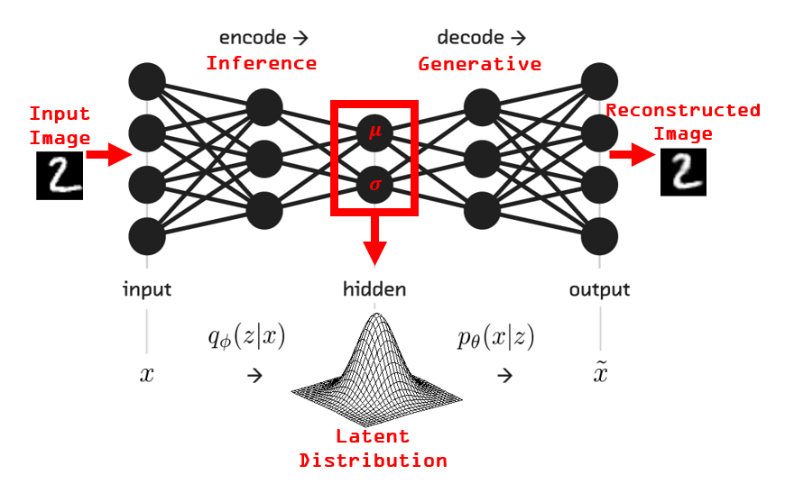
The VAE sets a unit diagonal Gaussian prior on the latent variable: \(p_{\theta}(z) = \mathcal{N}(0, I)\), and learns the distributions \(q_{\phi}(z \lvert x)\) and \(p_{\theta}(x \lvert z)\) jointly in a single neural network. The first half of the network that maps data into a distribution over latent space is known as the probabilistic encoder. The second half of the network that maps samples from the latent space back into the original space is known as the probabilistic decoder.
From the ELBO objective to a PyTorch loss function
In this section we will walk carefully from the theoretical ELBO objective function to specific PyTorch commands. We will focus on the objective one term at a time.
First term (reconstruction)
The first term of the ELBO objective is the expected reconstruction probability:
\[\mathbb{E_{q_{\phi}(z \lvert x)}} \log p_{\theta}(x \lvert z)\]Since the data is binary in this experiment, we will construct \(p_{\theta}(x \lvert z)\) to model a multivariate factorized Bernoulli distribution. (Note, the distribution chosen to model the reconstruction is dataset-specific. If you have continuous data then a diagonal Gaussian may be more appropriate.) This means that, for each data point, we view the 784 binary pixels values as independent Bernoulli observations. As such, the decoder network will output 784 Bernoulli parameters. The Bernoulli parameter is the probability of success in a binary outcome trial \(p \in [0, 1]\) (e.g., the probability of heads when flipping a biased coin).
Let’s take the \(j^{th}\) pixel of the \(i^{th}\) image as an example and call it \(x_{ij}\). Since we’re dealing with binary pixel values, \(x_{ij} \in \{0,1\}\) can be interpreted as the result of a Bernoulli trial. The model’s output will be the Bernoulli parameter corresponding to that pixel; let’s call that specific output \(p_{ij} \in [0,1]\). The likelihood of that pixel \(p_{\theta}(x_{ij} \lvert z_i)\) is then given by the Bernoulli PMF:
\[p_{ij}^{x_{ij}}(1-p_{ij})^{1-x_{ij}}\]Since the first term in the objective deals with the log probability, we can write the log likelihood instead:
\[x_{ij} \log p_{ij} + (1-x_{ij}) \log (1-p_{ij})\]This equation may look familiar. The negative of it is commonly known as binary cross entropy and is implemented in PyTorch by torch.nn.BCELoss.
Now, the log likelihood of the full data point \(x_i\) is given by
\[\begin{align} \log p_{\theta}(x_i \lvert z_i) &= \log \prod_{j=1}^{784} p_{\theta}(x_{ij} \lvert z_i) \\ &= \sum_{j=1}^{784} \log p_{\theta}(x_{ij} \lvert z_i) \\ &= \sum_{j=1}^{784} \bigg[ x_{ij} \log p_{ij} + (1-x_{ij}) \log (1-p_{ij}) \bigg] \end{align}\]In PyTorch the final expression is implemented by torch.nn.functional.binary_cross_entropy with reduction='sum'. Since we are training in minibatches, we want the sum of log probabilities for all pixels in that minibatch. This is accomplished by simply passing full batches through the same function call. You can think of the operation performed as first summing the 784 values for each datapoint and then summing over data points in the batch. In reality, a (batch_size, 784) size tensor of cross entropy values will be computed and then summed over all axes.
The expectation of the log likelihood over \(q_{\phi}(z \lvert x)\) is satisfied by simply sampling one point from \(q_{\phi}(z \lvert x)\) and passing it through the decoder. Note that there are no additional complexities here; this is a basic forward pass. As discussed in the previous post, this is the Monte Carlo approximation of the expected value of a function.
Second term (KL divergence, regularization)
The second term of the ELBO objective is the negative KL divergence between the variational posterior and the prior on the latent variable \(z\):
\[-KL[q_{\phi}(z \lvert x) \lVert p_{\theta}(z)]\]Since we have defined the prior to be a diagonal unit Gaussian and we have defined the variational posterior to also be a diagonal Gaussian, this KL term has a clean closed-form solution. The solution is essentially just a function of the means and covariances of the two distributions. The negative KL term simplifies to
\[-\frac{1}{2} \sum_{j=1}^{J} (1 + \log \sigma_j^2 - \mu_j^2 - \sigma_j^2)\]Where \(J\) is the size of the latent space (number of dimensions), and \(\mu\) and \(\sigma^2\) are the mean and variance vectors output from the probabilistic encoder.
In order to compute this, the forward pass of the network must also return mean and variance vectors output from the encoder, not just the reconstruction portion. In other words, the full model must return the outputs from both the encoder and the decoder.
The KL term can be computed across a minibatch with the following:
-0.5 * torch.sum(1 + logvar - mu.pow(2) - logvar.exp())
Where mu and logvar are tensors of means and log variances across the minibatch, respectively. Both of these tensors will have size (batch_size, latent_space_size).
Putting the terms together
In the following implementation, the binary cross entropy (BCE) and the KL divergence are calculated across the minibatch separately and simply summed at the end.
Sampling from the encoder
A key step in the flow of the VAE is sampling a data point from the encoder \(q_{\phi}(z_i \lvert x_i)\). The reparameterization trick is used to perform this sampling without introducing a discontinuity in the network (as discussed in the previous post).
\[z_i = g_{\phi}(x_i, \epsilon_i) = \mu_{\phi}(x_i) + diag(\sigma_{\phi}(x_i)) \cdot \epsilon_i \\ \epsilon_i \sim \mathcal{N}(0, I)\]In the forward pass, the vector of means and log variances are collected from the encoder. These vectors are used to generate a data sample as such
def reparameterize(self, mu, logvar):
  std = torch.exp(0.5*logvar)
  eps = torch.randn_like(std)
  return mu + eps*std
Experiment results
Data generation
At various points during training, I sampled a grid of points from the latent space. The points are linearly spaced coordinates on the unit square, transformed through the inverse Gaussian CDF. This results in a grid of points with evenly spaced quantiles of the Gaussian. In plain English (sort of), this means slicing the Gaussian into equal sized chunks.
from scipy.stats import norm
n = 20
self.grid_x = norm.ppf(np.linspace(0.05, 0.95, n))
self.grid_y = norm.ppf(np.linspace(0.05, 0.95, n))
The following gifs show the maturation of the model’s latent space and data generating capabilities at various points throughout training. At the beginning of the animations, the generated data are mostly noise. But as training (and the animation) progresses, you begin to recognize shapes. Keep in mind that the images you’re seeing here are essentially “fake”, in that they are not images from any dataset.
Animation throughout the entire training process:
![]()
Animation for just the early stages of training:
![]()
The final state of the learned manifold after training has completed:
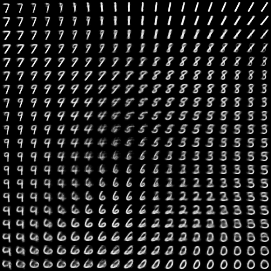
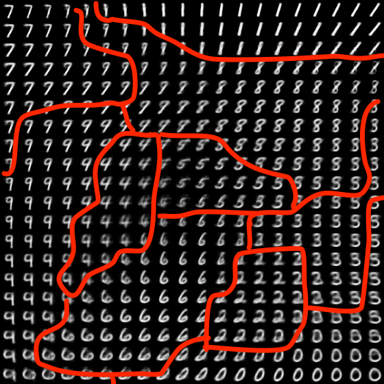
As you can see, there are regions dedicated to individual digits with smooth transitions in between. I tried hand drawing the boundaries between digits to aid the visualization:
Data reconstruction
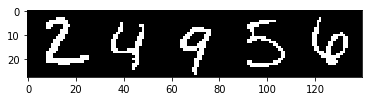
At various points throughout training I also tracked how well the model was reconstructing five hand-selected images:
The following animation shows how the model’s ability to reconstruct data improves over the training process:
![]()
Anomaly detection
Anomalous data can be detected by leveraging the probabilistic nature of the VAE. One way to detect anomalies is to measure the KL divergence between the encoder distribution \(q_{\phi}(z_i \lvert x_i)\) and the prior \(p_{\theta}(z)\) and compare it to the average across the training (or test) set.
I computed this KL divergence for every point in the training set and plotted the resulting distribution:
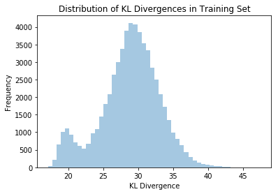
I then generated a noise sample:
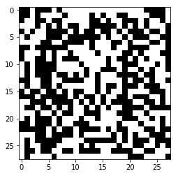
And calculated its KL divergence: 51.763. As you can see from the distribution plot, this value is a significant outlier and would be easy to detect using automated anomaly detection systems.
PyTorch Code
The data loading, data transformation, model architecture, loss function, and training loop are presented in this section. Detailed discussion on the key points of implementation are discussed above, but additional code annotation is provided for clarity. For the full code including visualization generation and experiment execution, please see this notebook on Github.
Imports and Helpers
import torch
import torch.utils.data
from torch.nn import functional as F
from torch import nn, optim
from torchvision import datasets, transforms
from torchvision.utils import save_image

from fastprogress import master_bar, progress_bar
import matplotlib.pyplot as plt
import numpy as np
from scipy.stats import norm
from pathlib import Path

import imageio

%matplotlib inline
Set configuration parameters for model training:
batch_size = 128
epochs = 10
seed = 199
log_interval=10
device='cpu'

torch.manual_seed(seed)
np.random.seed(seed)
Load and Prep Data
I added the lambda x: x.round() transformation to convert the images into binary form. We’re assuming the data likelihood to follow a Bernoulli distribution and this connection is more clear when the data is binary.
xforms = transforms.Compose([
    transforms.ToTensor(),
    lambda x: x.round()
])
I hand picked five images to use for visualizing reconstruction performance throughout training.
ds = datasets.MNIST('../data', train=False, transform=xforms)
recon_base_imgs = []
for i in [1, 4, 12, 15, 22]:
    img = ds[i][0]
    recon_base_imgs.append(img)
recon_base_img = np.concatenate([np.squeeze(x.numpy()) for x in recon_base_imgs], axis=1)
del ds

fig, ax = plt.subplots()
ax.imshow(recon_base_img, cmap='gray', interpolation='none')
plt.show()
Instantiate data loaders.
train_loader = torch.utils.data.DataLoader(
    datasets.MNIST('../data', train=True, download=True,
                   transform=xforms),
    batch_size=batch_size, shuffle=True)

test_loader = torch.utils.data.DataLoader(
    datasets.MNIST('../data', train=False, transform=xforms),
    batch_size=batch_size, shuffle=True)

len(train_loader.dataset), len(test_loader.dataset)
# (60000, 10000)
Define Model and Training Functions
The encoder and decoder modules are defined separately as VAEEncoder and BernoulliVAEDecoder, respectively. The BernoulliVAE class combines them to form the full model. It allows for a variable number of hidden layers and hidden layer sizes in both the encoder and decoder. It uses the ReLU activation function at each hidden layer.
class VAEEncoder(nn.Module):
    """
    Standard encoder module for variational autoencoders with tabular input and
    diagonal Gaussian posterior.
    """
    def __init__(self, data_size, hidden_sizes, latent_size):
        """
        Args:
            data_size (int): Dimensionality of the input data.
            hidden_sizes (list[int]): Sizes of hidden layers (not including the
                input layer or the latent layer).
            latent_size (int): Size of the latent space.
        """
        super().__init__()

        self.data_size=data_size

        # construct the encoder
        encoder_szs = [data_size] + hidden_sizes
        encoder_layers = []
        for in_sz,out_sz, in zip(encoder_szs[:-1], encoder_szs[1:]):
            encoder_layers.append(nn.Linear(in_sz, out_sz))
            encoder_layers.append(nn.ReLU())
        self.encoder = nn.Sequential(*encoder_layers)
        self.encoder_mu = nn.Linear(encoder_szs[-1], latent_size)
        self.encoder_logvar = nn.Linear(encoder_szs[-1], latent_size)

    def encode(self, x):
        return self.encoder(x)

    def gaussian_param_projection(self, x):
        return self.encoder_mu(x), self.encoder_logvar(x)

    def reparameterize(self, mu, logvar):
        std = torch.exp(0.5*logvar)
        eps = torch.randn_like(std)
        return mu + eps*std

    def forward(self, x):
        x = self.encode(x)
        mu, logvar = self.gaussian_param_projection(x)
        z = self.reparameterize(mu, logvar)
        return z, mu, logvar


class BernoulliVAEDecoder(nn.Module):
    """
    VAE decoder module that models a diagonal multivariate Bernoulli
    distribution with a feed-forward neural net.
    """
    def __init__(self, data_size, hidden_sizes, latent_size):
        """
        Args:
            data_size (int): Dimensionality of the input data.
            hidden_sizes (list[int]): Sizes of hidden layers (not including the
                input layer or the latent layer).
            latent_size (int): Size of the latent space.
        """
        super().__init__()

        # construct the decoder
        hidden_sizes = [latent_size] + hidden_sizes
        decoder_layers = []
        for in_sz,out_sz, in zip(hidden_sizes[:-1], hidden_sizes[1:]):
            decoder_layers.append(nn.Linear(in_sz, out_sz))
            decoder_layers.append(nn.ReLU())
        decoder_layers.append(nn.Linear(hidden_sizes[-1], data_size))
        decoder_layers.append(nn.Sigmoid())
        self.decoder = nn.Sequential(*decoder_layers)

    def forward(self, z):
        return self.decoder(z)


class BernoulliVAE(nn.Module):
    """
    VAE module that combines a `VAEEncoder` and a `BernoulliVAEDecoder` resulting
    in full VAE.
    """
    def __init__(self, data_size, encoder_szs, latent_size, decoder_szs=None):
        super().__init__()

        # if decoder_szs not specified, assume symmetry
        if decoder_szs is None:
            decoder_szs = encoder_szs[::-1]

        # construct the encoder
        self.encoder = VAEEncoder(data_size=data_size, hidden_sizes=encoder_szs,
                                  latent_size=latent_size)

        # construct the decoder
        self.decoder = BernoulliVAEDecoder(data_size=data_size, latent_size=latent_size,
                                           hidden_sizes=decoder_szs)

        self.data_size = data_size

    def decode(self, z):
        return self.decoder(z)

    def forward(self, x):
        z, mu, logvar = self.encoder(x)
        p_x = self.decoder(z)
        return p_x, mu, logvar
The loss function is discussed in detail above.
# Reconstruction + KL divergence losses summed over all elements and batch
def loss_function(recon_x, x, mu, logvar):
    BCE = F.binary_cross_entropy(recon_x, x.view(-1, 784), reduction='sum')

    # see Appendix B from VAE paper:
    # Kingma and Welling. Auto-Encoding Variational Bayes. ICLR, 2014
    # https://arxiv.org/abs/1312.6114
    # 0.5 * sum(1 + log(sigma^2) - mu^2 - sigma^2)
    KLD = -0.5 * torch.sum(1 + logvar - mu.pow(2) - logvar.exp())

    return BCE + KLD
Function to execute one epoch of training. This function also generates visualizations every figure_interval batches.
def train(epoch, mb, figure_interval, viz_helper):
    model.train()
    train_loss = 0
    pb = progress_bar(train_loader, parent=mb)
    for batch_idx, (data, _) in enumerate(pb):
        data = data.to(device)
        data = data.view(-1, 784)
        optimizer.zero_grad()
        recon_batch, mu, logvar = model(data)
        loss = loss_function(recon_batch, data, mu, logvar)
        loss.backward()
        train_loss += loss.item()
        optimizer.step()

        if batch_idx % figure_interval == 0:
            viz_helper.execute(model)

    return train_loss / len(train_loader.dataset)
Function to perform evaluation on the test set.
def test(epoch, mb):
    model.eval()
    test_loss = 0
    with torch.no_grad():
        pb = progress_bar(test_loader, parent=mb)
        for data, _ in test_loader:
            data = data.to(device)
            data = data.view(-1, 784)
            recon_batch, mu, logvar = model(data)
            test_loss += loss_function(recon_batch, data, mu, logvar).item()

    return test_loss / len(test_loader.dataset)
Function to fit the model over a number of epochs and generate visualizations.
def fit(model, epochs, figure_interval, viz_helper):
    mb = master_bar(range(1, epochs + 1))
    viz_helper.execute(model)
    for epoch in mb:
        trn_loss = train(epoch, mb, figure_interval=10, viz_helper=viz_helper)
        tst_loss = test(epoch, mb)
        mb.write(f'epoch {epoch}, train loss: {round(trn_loss,6)}, test loss: {round(tst_loss, 6)}')
VAE with 20-d Latent Space
Train a VAE with a 20 dimensional latent space. This VAE will be used to generate the data reconstruction visualizations.
viz_helper_20d = VAEVizHelper(recon_base_imgs, datagen_tracking=False)
model = BernoulliVAE(data_size=784, encoder_szs=[400], latent_size=20,
                     decoder_szs=[400]).to(device)
optimizer = optim.Adam(model.parameters(), lr=1e-3)
model

# BernoulliVAE(
#   (encoder): VAEEncoder(
#     (encoder): Sequential(
#       (0): Linear(in_features=784, out_features=400, bias=True)
#       (1): ReLU()
#     )
#     (encoder_mu): Linear(in_features=400, out_features=20, bias=True)
#     (encoder_logvar): Linear(in_features=400, out_features=20, bias=True)
#   )
#   (decoder): BernoulliVAEDecoder(
#     (decoder): Sequential(
#       (0): Linear(in_features=20, out_features=400, bias=True)
#       (1): ReLU()
#       (2): Linear(in_features=400, out_features=784, bias=True)
#       (3): Sigmoid()
#     )
#   )
# )
fit(model, 10, 10, viz_helper_20d)
Total time: 02:10 <p>epoch 1, train loss: 157.707501, test loss: 116.365121<p>epoch 2, train loss: 108.549474, test loss: 102.344373<p>epoch 3, train loss: 99.825192, test loss: 96.556084<p>epoch 4, train loss: 95.784532, test loss: 94.104183<p>epoch 5, train loss: 93.294786, test loss: 91.994745<p>epoch 6, train loss: 91.638687, test loss: 90.58567<p>epoch 7, train loss: 90.407814, test loss: 89.906129<p>epoch 8, train loss: 89.389802, test loss: 88.779571<p>epoch 9, train loss: 88.574026, test loss: 88.075248<p>epoch 10, train loss: 87.911918, test loss: 87.646744
VAE with 2-d Latent Space
Train a VAE with 2 dimensional latent space. This model will be used to generate the visualizations of data generation across the latent manifold. It is much easier to visualize a 2-d manifold.
model = BernoulliVAE(data_size=784, encoder_szs=[400,150], latent_size=2,
                     decoder_szs=[150,400]).to(device)
optimizer = optim.Adam(model.parameters(), lr=1e-3)
model

# BernoulliVAE(
#   (encoder): VAEEncoder(
#     (encoder): Sequential(
#       (0): Linear(in_features=784, out_features=400, bias=True)
#       (1): ReLU()
#       (2): Linear(in_features=400, out_features=150, bias=True)
#       (3): ReLU()
#     )
#     (encoder_mu): Linear(in_features=150, out_features=2, bias=True)
#     (encoder_logvar): Linear(in_features=150, out_features=2, bias=True)
#   )
#   (decoder): BernoulliVAEDecoder(
#     (decoder): Sequential(
#       (0): Linear(in_features=2, out_features=150, bias=True)
#       (1): ReLU()
#       (2): Linear(in_features=150, out_features=400, bias=True)
#       (3): ReLU()
#       (4): Linear(in_features=400, out_features=784, bias=True)
#       (5): Sigmoid()
#     )
#   )
# )
fit(model, 10, 10, viz_helper_2d)
Total time: 02:50 <p>epoch 1, train loss: 164.487584, test loss: 159.490324<p>epoch 2, train loss: 155.384058, test loss: 152.910404<p>epoch 3, train loss: 150.389809, test loss: 149.377793<p>epoch 4, train loss: 147.043944, test loss: 146.478713<p>epoch 5, train loss: 144.72857, test loss: 144.263316<p>epoch 6, train loss: 142.759334, test loss: 143.399154<p>epoch 7, train loss: 141.358421, test loss: 141.273972<p>epoch 8, train loss: 140.11891, test loss: 141.396691<p>epoch 9, train loss: 139.222043, test loss: 140.119026<p>epoch 10, train loss: 138.443796, test loss: 140.24413
Conclusion
In this post we drew the final connections between the abstract theory of variational autoencoders and a concrete implementation in PyTorch. By sampling a grid from the latent space and using the probabilistic decoder to map these samples into synthetic digits, we saw how the model has learned a highly structured latent space with smooth transitions between digit classes. We also discussed a simple example demonstrating how the VAE can be used for anomaly detection.
Resources
[1] PyTorch, Basic VAE Example