Variational Autoencoder Theory

This is the third post in my series: From KL Divergence to Variational Autoencoder in PyTorch. The previous post in the series is Latent Variable Models, Expectation Maximization, and Variational Inference and the next post is Variational Autoencoder Code and Experiments.

---

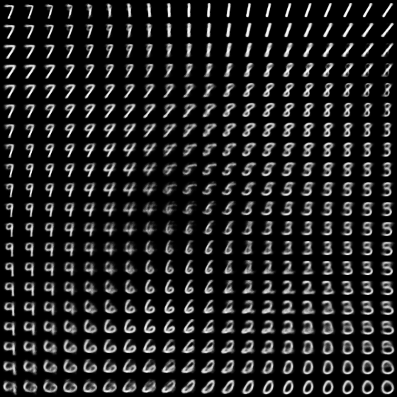
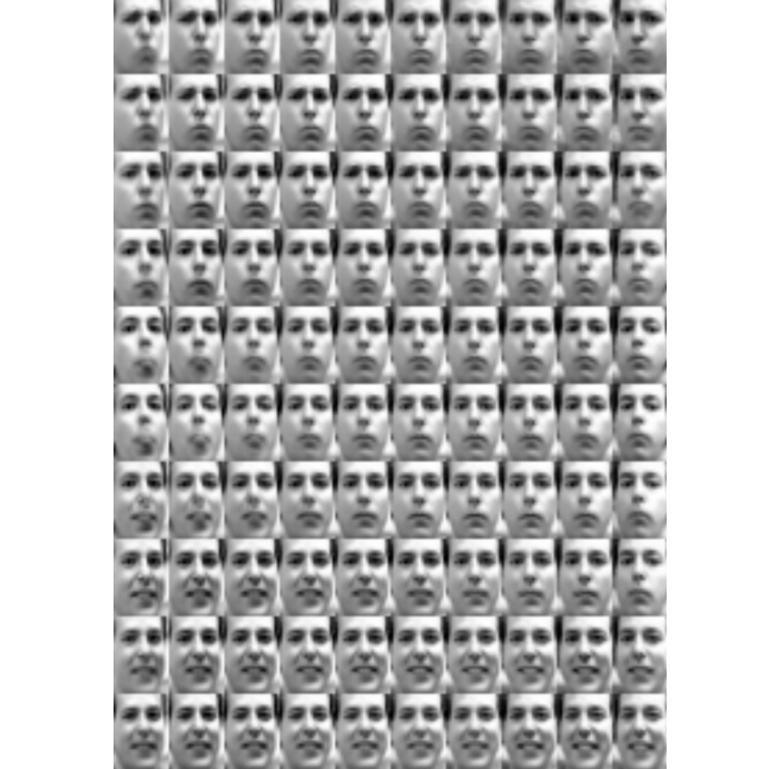
The Variational Autoencoder has taken the machine learning community by storm since Kingma and Welling’s seminal paper was released in 2013¹. It was one of the first model architectures in the mainstream to establish a strong connection between deep learning and Bayesian statistics. Quite frankly, it’s also just really cool. A VAE trained on image data results in the ability to create spectacular visualizations of the latent factors it learns and the realistic images it can generate. In the world of data science it’s an excellent bridge between statistics and computer science. It’s interesting to think about and tinker with, and it makes a great sandbox to learn and build intuition about deep learning and statistics.

(left) Synthesized digits from MNIST sampled from a grid on the learned latent manifold. Notice the smooth transitions between digits. (right) Synthesized faces sampled from a grid on the manifold of a VAE trained on the Frey Face dataset¹. Notice that the VAE has learned interpretable latent factors: left-to-right adjusts head orientation, top-to-bottom adjusts level of frowning or smiling.

It isn’t just a playground though; there are extremely valuable applications for the VAE on real world problems. It can be used for representation learning/feature engineering/dimensionality reduction to improve performance on downstream tasks such as classification models or recommender systems. You can also leverage its probabilistic nature to perform anomaly detection. Its data generation capability also lends itself to assist in the training of reinforcement learning systems.

The VAE seems very similar to other autoencoders. At a high level, an autoencoder is a deep neural network that is trained to reconstruct its own input. There are many variations of this fundamental idea that accomplish different end tasks, such as the vanilla autoencoder, the denoising autoencoder, and the sparse autoencoder. But the VAE stands apart from the rest in that it is a fully probabilistic model.

In this post we are going to introduce the theory of the VAE by building on concepts introduced in the previous post, such as variational inference and maximizing the Evidence Lower Bound (ELBO).

Table of contents:

1. Derivation of the VAE objective function
2. Intuition behind the VAE objective function
3. Model architecture
4. Optimization
5. Practical uses of the VAE

Derivation of the VAE objective function

As discussed in my post on variational inference, the intractable data likelihood which we would like to maximize can be decomposed into the following expression:

\[\log p_{\theta}(x) = KL[q_{\phi}(z) \lVert p_{\theta}(z \lvert x)] + \underset{z}{\sum} q_{\phi}(z) \log \frac{p_{\theta}(x,z)}{q_{\phi}(z)}\]

The focus of variational inference methods, including the VAE, is to maximize the second term in this expression, commonly known as the ELBO or variational lower bound:

\[\mathcal{L} = \underset{z}{\sum} q_{\phi}(z) \log \frac{p_{\theta}(x,z)}{q_{\phi}(z)}\]

In order to set the stage for the VAE, let’s rearrange \(\mathcal{L}\) slightly by first writing it as an expectation, substituting Bayes’ Rule, splitting up the logarithm, and recognizing a KL divergence term:

\[\begin{align} \mathcal{L} &= \underset{z}{\sum} q_{\phi}(z) \log \frac{p_{\theta}(x,z)}{q_{\phi}(z)} \\ &= \mathbb{E_{q_{\phi}(z)}} \log \frac{p_{\theta}(x,z)}{q_{\phi}(z)} \\ &= \mathbb{E_{q_{\phi}(z)}} \log \frac{p_{\theta}(x \lvert z)p_{\theta}(z)}{q_{\phi}(z)} \\ &= \mathbb{E_{q_{\phi}(z)}} \log p_{\theta}(x \lvert z) + \mathbb{E_{q_{\phi}(z)}} \log \frac{p_{\theta}(z)}{q_{\phi}(z)} \\ &= \mathbb{E_{q_{\phi}(z)}} \log p_{\theta}(x \lvert z) - KL[q_{\phi}(z) \lVert p_{\theta}(z)] \end{align}\]

Since \(q\) is intended to approximate the posterior \(p_{\theta}(z \lvert x)\) we will choose \(q\) to be conditional on \(x\): \(q_{\phi}(z) = q_{\phi}(z \lvert x)\). Now we’re ready to write down the objective function for the VAE:

\[\mathcal{L} = \mathbb{E_{q_{\phi}(z \lvert x)}} \log p_{\theta}(x \lvert z) - KL[q_{\phi}(z \lvert x) \lVert p_{\theta}(z)] \tag{1}\]

Intuition behind the VAE objective function

It’s easy to get get lost in the weeds here, so let’s zoom back out to the big picture for a moment: we want to learn a latent variable model of our data that maximizes the likelihood of the observed data \(x\). We have already shown that it is intractable to maximize this likelihood directly, so we have turned to approximating \(p_{\theta}(z \lvert x)\) with a new distribution \(q_{\phi}\) and maximizing the ELBO instead.

The practical items we would like to extract from this model are the ability to map data into latent space using \(q_{\phi}(z \lvert x)\) for exploration and/or dimensionality reduction, and the ability to synthesize new data by sampling from the latent space according to \(p_{\theta}(z)\) and then generating new data from \(p_{\theta}(x \lvert z)\).

Now, let’s begin unpacking the objective function by defining the prior on \(z\). The VAE sets this prior to a diagonal unit Gaussian: \(p_{\theta}(z) = \mathcal{N}(0, I)\). It can be shown that a simple Gaussian such as this can be mapped into very complicated distributions as long as the mapping function is sufficiently complex (e.g. a neural network)². This choice also simplifies the optimization problem as we will see shortly.

Next, let’s discuss the first term in the objective.

\[\mathbb{E_{q_{\phi}(z \lvert x)}} \log p_{\theta}(x \lvert z)\]

We want to learn two distributions, \(q\) and \(p\). The \(q\) we learn should be able to map data points \(x_i\) into a latent representation \(z_i\) from which \(p_{\theta}(x \lvert z)\) is able to successfully reconstruct the original data point \(x_i\). This term is something very similar to the standard reconstruction loss (e.g., MSE) used in vanilla autoencoders. In fact, under certain conditions, it can be shown that this term simplifies to be almost identical to MSE.

Simultaneously, the KL term is pushing \(q\) to look like our Gaussian prior \(p_{\theta}(z)\).

\[- KL[q_{\phi}(z \lvert x) \lVert p_{\theta}(z)]\]

This term is commonly interpreted as a form of regularization. It prevents the model from memorizing the training data and forces it to learn an informative latent manifold that pairs nicely with \(p_{\theta}(x \lvert z)\). Without it, the greedy model would learn distributions \(q_{\phi}(z \lvert x)\) with zero variance, essentially degrading to a vanilla autoencoder. By enforcing \(q_{\phi}(z \lvert x)\) to have some variance, the learned \(p_{\theta}(x \lvert z)\) must be robust against small changes in \(z\). This results in a smooth latent space \(z\) that can be reliably sampled from to generate new, realistic data, whereas sampling from the latent space of a vanilla autoencoder will almost always return junk⁵.

Model architecture

We choose \(q_{\phi}(z \lvert x)\) to be an infinite mixture of diagonal multivariate Gaussians

\[q_{\phi}(z \lvert x) = \mathcal{N}(\mu_{\phi}(x), diag(\sigma^2_{\phi}(x)))\]

Where the Gaussian parameters \(\mu\) and \(\sigma^2\) are modeled as parametric functions of \(x\). Note that \(\sigma^2\) is a vector of the diagonal elements of the covariance matrix. This choice provides us with a flexible distribution on \(z\) which is data point-specific because of its explicit conditioning on \(x\).

The VAE models the parameters of \(q\), \(\{\mu_{\phi}(x), \sigma^2_{\phi}(x)\}\), with a neural network that outputs a vector of means \(\mu\) and a vector of variances \(\sigma^2\) for each data point \(x_i\).

Similarly, the distribution \(p_{\theta}(x \lvert z)\) is modeled as an infinite mixture of diagonal distributions, where a neural network outputs parameters of the distribution. Depending on the type of data, this distribution is typically chosen to be Gaussian or Bernoulli. When working with binary data (like in the next post) the Bernoulli is used:

\[p_{\theta}(x \lvert z) = \mathcal{Bern}(h_{\theta}(z))\]

Where \(h_{\theta}(z)\) is an MLP mapping from the latent dimension to the data dimension. The output vector of \(h_{\theta}(z)\) contains Bernoulli parameters that are used to form the probability distribution \(p_{\theta}(x \lvert z)\).

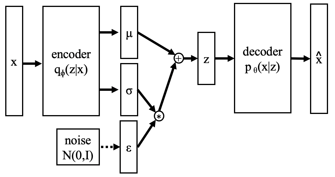
Distributions \(p_{\theta}(x \lvert z)\) and \(q_{\phi}(z \lvert x)\) are learned jointly in the same neural network:

Illustration of the VAE model architecture³

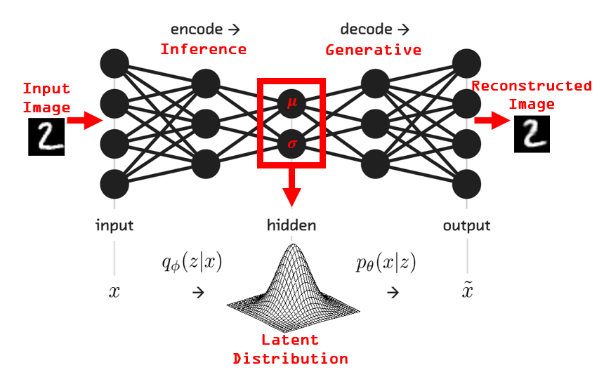
It is clear how the VAE model architecture closely resembles that of standard autoencoders. The first half of the network which is modeling \(q_{\phi}(z \lvert x)\) is known as the probabilistic encoder and the second half of the network which models \(p_{\theta}(x \lvert z)\) is known as the probabilistic decoder. This interpretation further extends the analogy between VAEs and standard autoencoders, but it should be noted that the mechanics and motivations are actually quite different.

The neural network weights are updated via SGD to maximize the objective function discussed previously:

\[\mathcal{L} = \mathbb{E_{q_{\phi}(z \lvert x)}} \log p_{\theta}(x \lvert z) - KL[q_{\phi}(z \lvert x) \lVert p_{\theta}(z)]\]

Optimization

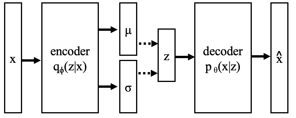
Let’s first describe the overall flow and inner workings of this neural network. Data points \(x_i\) are fed into the encoder which produces vectors of means and variances defining a diagonal Gaussian distribution at the center of the network. A latent variable \(z_i\) is then sampled from \(q_{\phi}(z_i \lvert x_i)\) and fed into the decoder. The decoder outputs another set of parameters defining \(p_{\theta}(x_i \lvert z_i)\) (as discussed previously, these parameters could be means and variances of another Gaussian, or the parameters of a multivariate Bernoulli). During training, the likelihood of the data point \(x_i\) under \(p_{\theta}(x_i \lvert z_i)\) can then be calculated using the Bernoulli PMF or Gaussian PDF, and maximized via gradient descent.

In addition to maximizing the data likelihood, which corresponds to the first term in the objective function, the KL divergence between the encoder distribution \(q_{\phi}(z \lvert x)\) and the prior \(p_{\theta}(z)\) is also minimized. Thankfully, since we have chosen Gaussians for both the prior and the approximate posterior \(q_{\phi}\), the KL divergence term has a closed form solution which can be optimized directly.

Performing gradient descent on the first term also presents additional complications. For one, computing the actual expectation over \(q_{\phi}\) requires an intractable integral (i.e., computing \(\log p_{\theta}(x \lvert z)\) for all possible values of \(z\)). Instead, this expectation is approximated by Monte Carlo sampling. The Monte Carlo approximation states that the expectation of a function can be approximated by the average value of the function across \(N_s\) samples from the distribution:

\[\mathbb{E_{q_{\phi}(z \lvert x)}} \log p_{\theta}(x \lvert z) \approx \frac{1}{N_s}\sum_{s=1}^{N_s} \log p_{\theta}(x \lvert z_s)\]

In the case of the VAE we approximate the expectation using the single sample from \(q_{\phi}(z \lvert x)\) that we’ve already discussed. This is an unbiased estimate that converges over the training loop.

Another gradient descent-related complication is the sampling step that occurs between the encoder and the decoder. Without getting into the details, directly sampling \(z\) from \(q_{\phi}(z \lvert x)\) introduces a discontinuity that cannot be backpropogated through.

Diagram of the VAE without the reparameterization trick. Dashed arrows represent the sampling operation.

The neat solution to this is called the reparameterization trick, which moves the stochastic operation to an input layer and results in continuous linkage between the encoder and decoder allowing for backpropogation all the way through the encoder. Instead of sampling directly from the encoder \(z_i \sim q_{\phi}(z_i \lvert x_i)\), we can represent \(z_i\) as a deterministic function of \(x_i\) and some noise \(\epsilon_i\):

\[z_i = g_{\phi}(x_i, \epsilon_i) = \mu_{\phi}(x_i) + diag(\sigma_{\phi}(x_i)) \cdot \epsilon_i \\ \epsilon_i \sim \mathcal{N}(0, I)\]

You can show that \(z\) defined in this way follows the distribution \(q_{\phi}(z \lvert x)\).

Diagram of the VAE with the reparameterization trick. Dashed arrows represent the sampling operation.

Practical uses of VAE

Probably the most famous use of the VAE is to generate/synthesize/hallucinate new data. The synthesis procedure is very simple: draw a random sample from the prior \(p_{\theta}(z)\), and feed that sample through the decoder \(p_{\theta}(x \lvert z)\) to produce a new \(x\). Since the decoder outputs distribution parameters and not real data, you can take the most probable \(x\) from this distribution. When the decoder is Gaussian, this equates to simply taking the mean vector. When it’s Bernoulli, simply round the probabilities to the nearest integer \(\in \{0, 1\}\). Note that for data generation purposes, you can effectively throw away the encoder.

Another practical use is representation learning. It is certainly possible that using the latent representation of your data will improve performance of downstream tasks, such as clustering or classification. After training the VAE you can transform your data by passing it through the encoder and taking the most probable latent vectors \(z\) (which equates to taking the mean vector outputted from the encoder). Data outside of the training set can also be transformed by a previously-trained VAE. Of course, performance will be best when the new data is similar to the training data, i.e., comes from the same domain or natural distribution. As an extreme example, it probably wouldn’t make much sense to transform medical image data using a VAE that was trained on MNIST.

Yet another use is anomaly detection. There are various ways to leverage the probabilistic nature of the VAE to determine when a new data point is very improbable and therefore anomalous. Some examples:

• Pass the new data through the encoder and measure the KL divergence between the encoder’s distribution and the prior. A high KL divergence would indicate that the new data is dissimilar to the data the VAE saw during training.
• Pass the new data through the full VAE and measure the reconstruction probability. Data with a very low reconstruction probability is dissimilar from the training set.
• With some additional work it’s possible compute the actual log likelihood \(\log p_{\theta}(x)\) for new data. This approach requires leveraging importance sampling to efficiently compute a new expectation. Look out for more details on this approach in a future post.

Conclusion

In this post we introduced the VAE and showed how it is a modern extension of the same theory that motivates the classical expectation maximization algorithm. We also derived the VAE’s objective function and explained some of the intuition behind it.

Some of the important details regarding the neural network architecture and optimization were discussed. We saw how the probabilistic encoder and probabilistic decoder are modeled as neural networks and how the reparameterization trick is used to allow for backpropogation through the entire network.

To see the VAE in action, check out my next post which draws a strong connection between the theory presented here and actual PyTorch code and presents the results of several interesting experiments.

Resources

[1] Diederik P. Kingma, Max Welling, Auto-Encoding Variational Bayes

[2] Carl Doersch, Tutorial on Variational Autoencoders

[3] Rebecca Vislay Wade, Visualizing MNIST with a Deep Variational Autoencoder

[4] Volodymyr Kuleshov, Stefano Ermon, The variational auto-encoder

[5] Irhum Shafkat, Intuitively Understanding Variational Autoencoders

[6] Daniil Polykovskiy, Alexander Novikov, National Research University Higher School of Economics, Coursera, Bayesian Methods for Machine Learning

[7] Martin Krasser, From expectation maximization to stochastic variational inference